Glaciation; Global Warming; Long Term Climate Change;  Temperature;  CO2; Earth  Magnetic  Fields;  Solar Wind; Dendrochronology of Bristlecone Pines, German Oak from Spessart and Trier Forest, Chile, and Java;  correlated with Solar Activity, Sun Spots,  El Niño  and  La Niña Events, Drought in Africa, and Egyptian Chronology

 

                                    James H. L. Lawler  July 1998 ã

 

There are a number of connected broad events that are usually looked upon as separate specialties but which in truth are intimately interconnected.  The dendrochronology is an isolated specialty within botany, but the tree ring growth patterns reflect the weather, which in turn is a strong reflection of climatic changes such as the El Niño and La Niña events. The weather is another isolated specialty.  But all of this correlates nicely with the number of sun spots appearing on the sun, usually assigned to a special study within astronomy. The number of spots has varied recently from a very few, 7 for example in December of 1997, to a high of about 150 to even 200 on an “11 year” cycle.  This cycle also is often plotted as “The Hale 21 year cycle”, by plotting every other cycle “upside down” (in computer usage we multiply the number of spots by -1).  We do this because the spots come in magnetic pole pairs, with a north magnetic pole leading a south magnetic pole, in one cycle, but a south leading north in the next set of sun spots. The Hale presentation gives a  representation of the fact that every other cycle has this N-S  inversion.

 

The real solar cycles also start at high solar latitudes and move inward toward the solar equator, in a “butterfly pattern”, but that does not effect the Earth so much as the pure number of spots or more properly the fraction of the sun covered with them.  Between 1600 and 1700 AD the sun underwent a “quite phase”, the number of sun spots fell to an unusual low, frequently zero. This resulted in unusual cooling of Earth by about 2 degrees C.;  a “little ice age”  also called the Maunder Minimum.  For example the canals in Holland froze over solid for the first time, allowing writing of “Hans Brinker and the Silver Skates” and people changed sleeping habits etc. to accommodate this  cold period.  But this is not the first such  climatic cold  period.  There were others at 1450 AD called the Spörer Minimum, at 1250/1280 AD which with its associated drought caused the collapse of the Mesa Verde / Anasazi,  and Wari cultures,  and at about 600 AD.  The C-14 data of Eddy documents these Solar / Earth events as well as others in 400 BC, 700 BC, 1350 BC, with mild drops at 2000 BC  and 2400 BC etc.  There are also 100 year cycles modulating  the 10.57 year solar cycles.

 

Periods of  high solar sun spot activity tend to be warm, and periods of low activity tend to be cool.  The low activity,  cooling the earth at solar sunspot minima, always is related to an El Niño event.  There are other El Niño events between minima, but every minima has an El Niño event associated with it.   El Niño appears to be a way of the ocean adding heat from the ocean to the atmospheric system to minimize the overall change (La Chatlier’s principle). The La Niña events tend to be associated with maximal activity, and they usually are linked to an El Niño: -- they come either before or more commonly just after an El Niño event - particularly the year following a strong event.  These events are worldwide in scope.  There is a mild wet winter in Texas, excess water including mud slides in California, and flooding in Peru, and Mexico, but drought in Java, Australia,  and Africa, and a summer drought in much of the southern USA and a monsoon failure in India with a resulting drought / crop failure there. The summer after an El Niño event seems to be hot and dry, with crop failures and a bad year for tree growth almost worldwide.  These events are recorded in the tree rings of California, Java, Germany,  and  Chile.

The trees give us a record that goes far before the recorded history of El Niño  Southern Oscillation (ENSO) events.  We have complete good records since 1877, with spotty records getting fewer and worse back to 1554. The earlier records are deduced from anecdotal notes in diaries etc. not actual deliberate scientific data, but most are quite reliable.

 

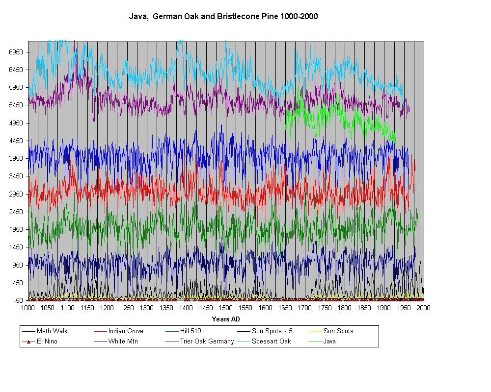
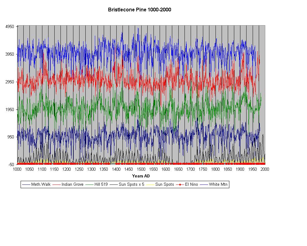
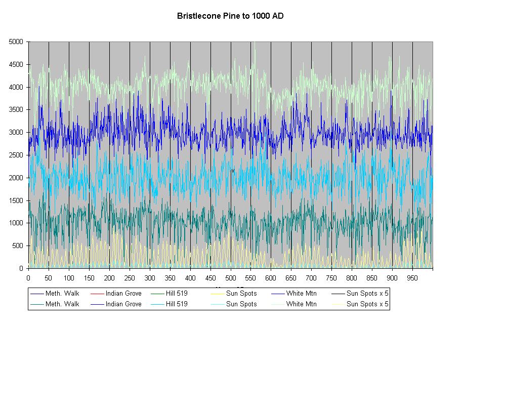
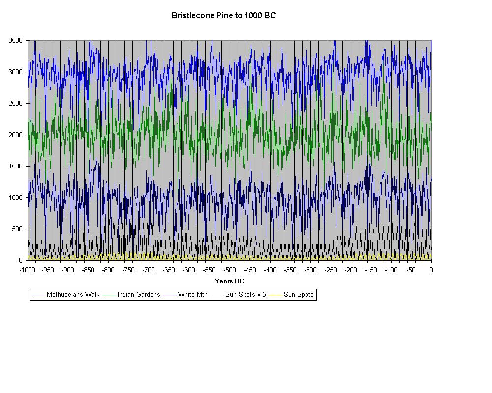
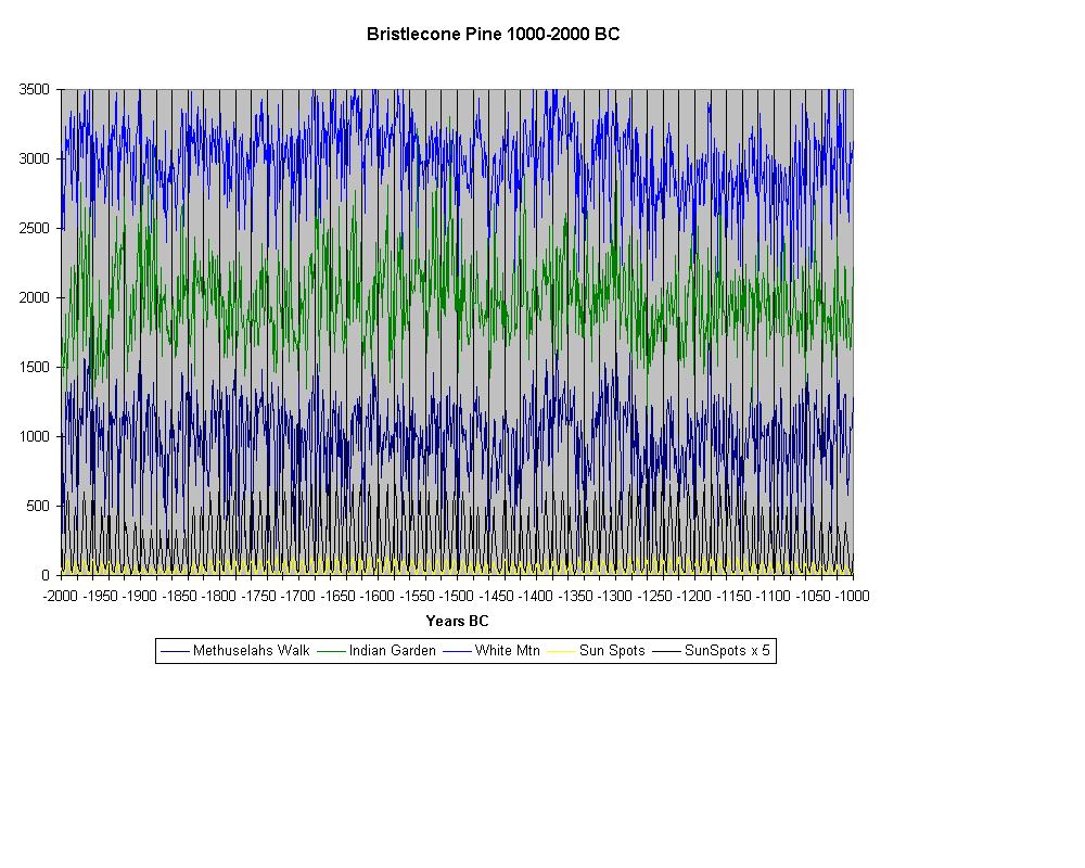
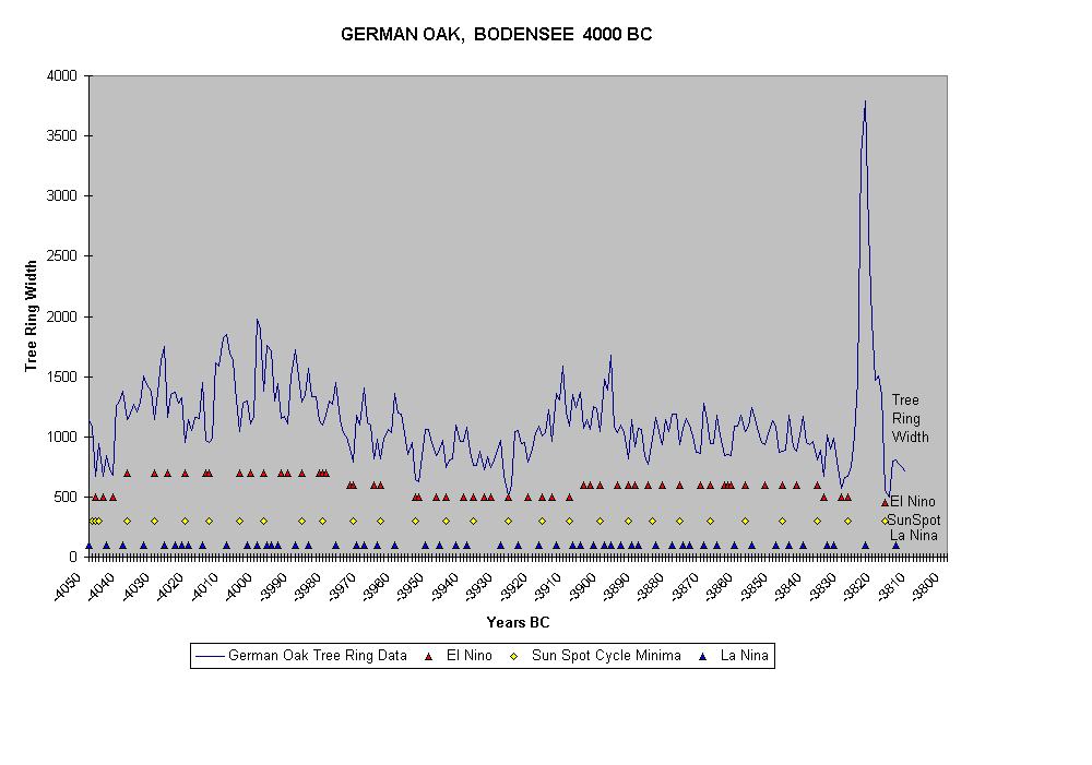
There are a few rules that allow us to convert tree ring dendrochronology records from the Bristlecone Pines (BCP) of Nevada and California into reasonably certain records of El Niño and La Niña events.  The first step is to note that the year after a solar sun spot minimum always is an El Niño event and also a bad tree ring year with lower than usual growth.  This was first seen for the Oak forest data from Spessart and Trier in Germany, and thus this allowed using these low spikes to synchronize the minima.   It is observed that  from 1700 to 1995 the solar minima are observed to be an average of 10.57 years apart, but there is some variation in this and 9, 10, 11, or 12 year cycles all are possible.  Most are either 10 or 11 years.  Going backward it is possible to insert a new tree ring minima roughly 10 years prior to a known data point, and to synchronize these with tree ring minima, and insist that over long periods, such as a century,  that they must average very near 10.57 years.  This allows us to work backward cycle by cycle.  Since we have many tree ring data sets from present back to 1000 AD this allows relative certainty, and we do not need to use all the available data. The Chilean dendrochronology for example has been used to check the other data- just to be sure.  But from 1000 to 1 AD there are fewer and fewer locations with tree ring observations and finally prior to 1 BC there are only three major BCP sites of record. These records go back continuously to  6000 BC (Methuselah’s Walk), to 5141 BC (White Mountain Master Chronology), to 2370 BC (Indian Garden) with Mammoth, Hill 519 reported from 1 AD to 1979.  There are other Scots Pine records of sub-fossilized trunks found in bogs from Finland and Sweden, and other Oak going back to Roman times from German and Netherlands, but these - I am ashamed to say - have not been made easily available. The main tree ring records may be  found on the Internet at the NOAA  International Tree Ring Data Bank (ITRDB) site at http:\\www.ngds.noaa.gov/paleo/treering.html. The German Oak are from B Huber (1949) et.al.  I have literature stating that he had records to 9000 BP (7000 BC) but those are not available to me at this time. In making decisions, we should insist that a strong majority of BCP meet the small or large criteria.  Earlier I had used only the two German Oak lists and both had to have bad years before deciding it was an El Niño year. The Java data reinforced the German analysis. The BCP allowed adding a few El Niño events that had not been “both” with the German Oak data.

 

There also are two other data items that were entered in making the first long range ENSO projections. The Japanese recorded seeing Aurora borealis events on occasion and that had to be a maximum activity time. The Aurora is not seen as far south as Japan unless it is a major event The Chinese and Japanese also reported naked eye (with smoked glass) solar sun spot activity on occasion  and these data were collected by Kanda (1933) and Matsushita (1956) and those 50 or so sightings going back to 33 BC were used to synchronize sun spot maximal events.  With that it was possible to synchronize the 10.57 year cycle for about 2000 years. With the solar pattern established also it was possible pin point minimum El Niño events for this same time.  The frequency of or number of sightings in any time period or absence allowed estimation of the number of sun spots at peak.  This also had to match the C-14 data of Eddy (see Sci American 1976) to give the envelope (modulation) of the SS values.  Known cold periods such as the Maunder minimum for which we have real observations, were also replicated for the Spörer Minimum at 1400 AD, and the known cold period / drought at about 1250 AD, and 600 AD etc.  Thus even the modulation can be recreated with confidence.  With 7 tree ring data files the; 4 BCP and the other 3, the analysis added a numerous more “in between” probable ENSO events. Where all or most tree rings were unusually small ENSO  events were shown. Where all or most tree rings were unusually large La Niña events were shown This for the first time allowed confident selection of  La Niña events from universal appearance of large rings .  As the selection dropped to only three BCP tree ring data sets before 1 AD the  probability of correct analysis dropped, and no doubt some detail has been lost.  Some  unexpected clear strings of events unlike the oscillatory events  in more recent times were observed, but these also match Egyptian reported strings of “good” and “famine / drought” crop  years,  so are shown as deduced.

 

With this data we present a list of probable ENSO  events for more than 4000 years with more than 1000 entries. compared to 130 to 200 years with  about 50 - 100 listed entries in  the recent literature.

 

Tree ring data also has been used to date tsunami events. From Tlinket Indian legends there was a major tsunami in the Washington state, but no exact date could be assigned. Their legend said that the ground shook, (with hands always showing an up and down THEN a sidewise shake in that sequence) followed by a “grandfather wave”, (gesture hands rolling over heads). This was found to have killed some cedar trees about 30 Km inland, and looking at the tree rings the date could be placed with precision to Jan to March 1700. The tree rings showed clear sequence up to 1699 which was complete but the spring growth had not begun for 1700, thus dating the tsunami.

 

There are  several other types of data that can contribute to the information.  We have used dendrochronology as the primary tool, but glacial ice cores as mentioned below also give the same sort of information.  From the year by year accumulation of ice, and countable annual ring in the Greenland glaciers going back 7 million years we have a year by year record of climate, etc.  The oxygen 18 isotope ratio, carbon dioxide fraction, and C-14 isotope ratios all tell stories of temperature,  and sun activity. But even more importantly dust and pollen trapped also tell stories of climate, volcanic activity and wind conditions.  Particularly the volcanic activity is useful and can be used to link synchronous events in several different locations.  There are also ice cores from Peru,  Antarctica and Switzerland glaciers on the Internet now.

 

In addition to glaciers, the lake bottom silt precipitation has annual layers, and these Varves can also tell the same sort of story.  I would be VERY interested in the lake Titicaca  varve record which I do not believe has been properly done and reported at this time.  It is of such major size that a good consistent record  probably could be made.  The Varve record can also include pollen trapped and the size and consistency tell climatic stories.  Similarly Sea bottom deposits, particularly at deltas, can be used.  On a very long term basis lava flows show magnetic polarity changes, and  any fire such as a hearth fire can lock in the magnetic pole configuration for clay heated past the annealing point.  That also allows TLD (Thermo-luminescent- dating) of the sample since radiation induced crystal distortions flash with luminescence as they are annealed in the present and the number of light flashes tells the age since last annealing.  This technique supplements radio carbon dating and in places is better,  covering a different range of time.

 

 

 

 

GLACIATION

 

There have been several period of major glacial activity recorded in the geological record. Starting with some of the very oldest rocks the Huronian Glacial record was at 2500 to 2100 MA (MA = Millions of Years Ago Millions Años) 2 billion years ago. This was followed by the Stuartian-Verangina at 950-600 MA, The  Andean-Sahara Ice Age at 450-420 MA,  The Karoo “Permian” at 360-260 MA and the “recent” Cenozoic set starting about 30 MA. There have been 5 distinct recent periods of Glaciation,  “recent” being in geological terms.  The last of these ended about 18,000  years ago.  The weather  in those periods as determined by ice core samples shows occasional  swings of  10-18 degrees C in just one decade, compared to the 2 degrees C in the Maunder minimum.  Even more interesting is the start of one ice age where the English Channel froze solid in just 12 years,  with a world wide drop of about 18 degrees C in  less than two decades!  Several such extreme swings,  some up,  some down,  are recorded.  It boggles the mind as to how we would contend with such a swing today!  The temperature is found from analysis of an isotope of Oxygen, O-18,  and we also can obtain CO2 (Carbon Dioxide) levels from trapped gasses,  as well as volcanic dust, and spore, pollen samples, etc.  all of which tell climatic stories.  Perhaps the best of these samples is the Russian VOSTOK sample  from Greenland which goes back continuously 7 million years layer by layer.  Several other U.S. Arctic and Antarctic cores collaborate this data making it extremely credible.

 

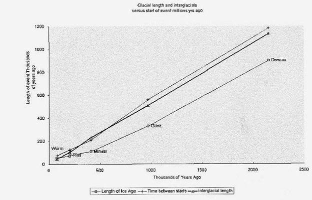
GLACIAL   AGES AND INTERGLACIAL  PERIODS

 

2,150,000 BP   Start Doneau Glacial age      1,250,000      End Doneau Glacial

                                                                                                     Start Villafranchian Interglacial

 970,000    End Villafranchian Warm                   640,000     End Günz Glacial

                    Start  Günz  (Nebraska) Glacial                            Start Aftonian  Interglacial

 

410,000   End  Aftonian  IG                                   300,000      End Mindel

                  Start Mindel (Kansasian) Glacial                            Start  Yarmouth  IG

 

 200,000   End  Yarmouth  IG                                120,000        End Riss Glacial

                Start Riss (Illinoisian) Glacial                                       Start Sangamon  IG

 

   75,000     End  Sangamon  IG                              21,000         End Würm Glacial

                    Start Würm (Wisconsian) Glacial                   Start present Interglacial Warm period

 

Table  of glacial periods, listing start date and ending dates,  and interglacial periods.

 

The long term climatic data shows a series of  5 major glacial periods, with 5 interglacial periods,  each usually subdivided with warm interstitial periods in the glacial times and cold periods in the interglacial.  Overall they all are getting sorter in duration, i.e. closer and closer together.  These are shown in a table above. The more interesting thing about this is when duration is plotted against age  (below) these show a straight line, allowing us to predict the start of the next ice age. 

The next ice age is due more or less any time now as the digital analysis predicts 18,600 years for our  interglacial,  which started either 18,000 BC or  18,000 years ago (BP); but the probable error is at least ± 500 years and realistically about ± 1000 years variation. The key point is we are due within the limits of prediction for the trigger start of a glacial period at any time.

 

 

The table above does not show the interstitial periods and there is a clear relationship of the complete system to the variations in Earth’s orbit. These Milankovitch cycles correspond to a 23,000 year precession of the Earth’s pole, often called the precession of the equinoxes;  in addition there is a 41,000 year cycle in the tilt of the earth pole; and finally a 100,000 year change in the eccentricity of the orbit from nearly circular to about 5% eccentricity.  These cycles closely control the relative volume of ice in the glaciers.  However, these variations are set against an overall cooling trend that started about 55 to 65 million years ago with the start of the Cenozoic period. This trend has seen Earth loose about 12 degrees C  worldwide, from 20 C to 8 C (42° N) with a loss of about 2° C from 1 million years ago to 20,000 years ago.  Then about 10,000 years ago at 8,000 BC there was a sharp rise of 15° C from 6° C to an average of about 21° C. 

This warm plateau has persisted for 10,000 years with only a  minor shift of up to ± 2° C maximal change in that entire time.  This long steady plateau of warm temperature is in sharp contrast to major 12-15° C temperature swings in the prior 40,000 to  1,000,000 years,  and the  somewhat smaller 6 to 8° C swings from 1 to 20 million years ago.  We do NOT live in “normal” times, relative to the last geologic ages. 

 

Humanity has grown and prospered under this unusual warm period, but there is no guarantee it will last;  in fact based upon the known temperature record I can virtually guarantee it cannot last.   The only question is not IF but WHEN the next major ice age will occur.  Based upon the historical record we should be much more worried about a sudden rapid cooling to the past “normal” temperature about 15° C lower than present; much more than global warming! In fact any global warming may be a blessing in rather heavy disguise.  It may be holding off a trigger event that is just waiting to start an ice age.

 

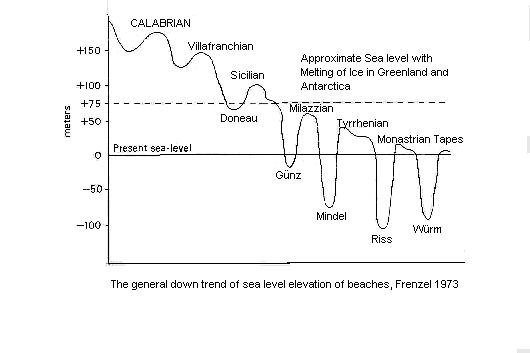
Sea levels also follow  Glaciation patterns.  As Glaciers form they tie up huge quantities of water, literally thousands of cubic kilometers of water,  and sea levels fall. Conversely as glacial ice melts sea levels rise. 

 

There are records contained in the beach levels of the world of 7 glacial periods, more than just the 5 glaciers for which we have good land records. If the West Antarctic sheet, the smaller half, alone melts,  that will result in about a 15 meters rise in sea level.  A 15 meter rise perhaps could be handled.  Dikes such as are used in Holland  could be used to prevent flooding of low coastal cities.  If the Antarctic sheet totally melts the sea level will rise about 42 meters.  If both Antarctica and Greenland melted we would see about 75 meters rise! In the last cases this would be a potential catastrophe. The larger 42 to 75 meter rise would flood large areas including most major coastal cites like New York, Philadelphia. Washington DC, Miami (in fact Florida including Disney World virtually disappears - totally!),  San Diego, Los Angles, San Francisco, the inner California valleys flood, Seattle, Melbourne, Sidney, Tokyo,  Hong Kong,  all of Malaysia most  of Java including Jakarta,  numerous Pacific atoll islands, Bombay, Calcutta, Capetown, most of the major cities in South America (Lima overall would escape, but Callao would be gone),  etc.  The mouth of the Amazon, Mississippi, and Nile Rivers etc. all flood for many km inland - in one case 2000 Km inland.  Hundreds of millions of people, perhaps 2 billions of people would be displaced.

 

This hot cycle could also cause a return of the great deserts of the past. The effect on arable land could be overwhelming. At one time the US had a desert that stretched from Dakota to Arizona and it was 2000 Km wide.  Later in Geological time the kilometer thick (3000 foot) petrified desert of the Navajo sandstone is a relic of another desert that covered most of what is now Arizona, Utah, New Mexico, and parts of Colorado and Nevada. The Sahara has been expanding in any case, and the Gobi could grow to massive proportions covering the grassy steps of mid central Asia and East Europe. Thus a major global warming can be almost as bad as an ice age.

 

The greenhouse effect “Global warming” scare is not based upon sound science. In fact it is based upon political premises designed to allow politicians put a hand into your pocketbooks by scare tactics, (a polite way of saying governmentally sponsored theft). There is  an overall very close link between the CO2 level and temperature of the Earth.  This has been measured on both a short term (150 year) basis, and over geological (65,000,000 year) basis.  The two do track one another.  BUT......  a closer evaluation of the data shows that the temperature first rises or falls and then the CO2 level follows.  The temperature is causative and the change in CO2 level is the effect.  There is a clear scientific reason for this. 

 

As liquids are heated the gasses dissolved become less soluble,  and as liquids are cooled the gasses become more soluble in general.  The quantity of CO2 dissolved in the oceans is  MUCH more than the quantity of CO2 in the atmosphere.  The CO2 in the air is about 380 ppm (0.00038 fraction) of the column of air which has a total weight at any point of a surface pressure of 76.0 cm of mercury, or based upon a centimeter square of earth’s surface and knowing mercury is 13.6 grams per cc, we find 1034 grams of air or  0.39 grams of CO2. The ocean has  dissolved in it 8.8% carbonates.  Not all can be released as CO2 but there is roughly  1% releasable CO2.  This a very much a “water world” -75% of the surface is water, and the oceans average about 3-4 km depth based on world wide coverage or 3+ metric tonnes per sq.cm.  That is 30 to 40 Kg of releasable CO2 per sq.cm., some  8000 + times more CO2 in the oceans than in the air.

 

As the earth warms up, the oceans warm up also, releasing CO2 into the atmosphere.  The CO2 was less soluble in warm water.  As the oceans cool they can adsorb more CO2 from the air, lowering the CO2 level in the atmosphere.  This is a simple freshman chemistry calculation. and the cause - effect observed levels over VERY long periods follow this simple concept.  Other factors such as our prolific dumping of CO2 into the air can temporarily alter the equilibrium, but  there is no observational basis for the greenhouse effect.  Even should it happen it is something we can deal with and control far more easily than Glaciation.

 

There is one more factor involved in this fraud.  The CO2 does have infra red adsorption bands that might block re- radiation of heat.  But those bands are covered up by the IR. adsorption bands of water!   There is FAR more water in the air than CO2 (roughly 25 times more). Depending on humidity and temperature the air holds of the order of magnitude of 1% water (40% humidity at 20 degrees C), compared to 0.038% CO2.  

 

The effect of moisture on heat radiation is commonly observed.  Moist air does hold in heat at night far better than dry air.  Desert temperatures commonly drop 20 to 25 degrees C between day and night and extremes of 40 degrees C occur in such places as the Gobi desert and Alto-plano. In moist climates, such as coastal cities like Lima, or New York, or London, the day night swing is about 10 degrees C; usually a bit less.  Thus moisture has an order of magnitude more effect than the CO2, and completely masks any possible effect from CO2. This; however, give much greater credence to preservation of Rain forests, to add moisture to our atmosphere, and to help the man caused desertification of the globe. This global disease has caused the major expansion of the Sahara and drying out of  millions of square km or grass land by overgrazing in Africa,  and is now causing the loss of productivity in Amazonia, which globally can be catastrophic.  The conversion of forest to poor quality pasture  yields momentary gain and long term disaster.

 

What does cause the changes in temperature?  Obviously climatic swings occur seasonally by changes in insolation,  the quantity of sun light striking the surface.  But globally, what causes non-seasonal long term trends?  The surprise answer appears to be change in the magnetic field of the earth precede temperature changes by almost exactly 3 years. If we look at measured gammas of magnetic field intensity  and temperature changes offset by that three year lag, the two curves follow one another too closely to be chance. They are mirror images of one another.  That begs an explanation of why this happens - does the magnetic field cause temperature change and if so HOW. Even more  perplexing what causes magnetic field gamma to change?

 

There also is another possibility, that both temperature and magnetic fields are being changed by some third causative change, and they are both symptoms of that cause.  We know that temperature does not cause magnetic change, the delay precludes that. There have been numerous magnetic field N-S to S-N reversals of the magnetic field of the entire earth over geological time, and these magnetic filed reversals frequently coincide with major temperature swings.  In fact all of the initiations of glacial period coincide with a magnetic reversal. Thus the link of Magnetic field  change to Temperature change is substantiated for both short and very long range events.

 

Recent measurement show that the magnetic field shrinks or expands in response to the solar wind.  If the sun is active, producing a major solar wind, then this pushes the magnetopause  down  towards the Earth,  making the magnetic field more “concentrated” increasing gammas.  As the sun has lower solar wind the magnetopause expands outward allowing the magnetic field more room and the gammas drop.  Since the solar wind is released from the sun many hours before we see the two effects,  we know the solar wind causes the change in magnetopause and field density.

 

But that does not account for temperature changes.  The high field also correlates with high aurora borealis (or aurora australis).  While the light from those displays are minor compared to the energy directly from the sun at high noon, they strike the Earth at a place where there is little or no direct insolation. In fact the aurora at maximum can be bright enough to read a newspaper in the middle of the arctic night.  The energy input at that time and place may have an unusual effect on overall climate. In particular it may prevent triggering Glaciation. 

 

The albedo of the land part of Earth overall is about 0.30. The albedo over water is about 0.10, i.e. water adsorbs about 90% of all energy that strikes it.  Land overall adsorbs 70%.  But the albedo of snow,  particularly fresh snow, runs 80-90% meaning that it adsorbs only 10 to 20 % with 15% being a good estimate overall.  “Dirty” snow reflects 70% adsorbing 30% of the insolation.  Thus a snow field rejects incoming heat,  and a glacial field once started cools the area near it allowing the snow to persist.

 

A glacial cold zone once formed builds rapidly. If snows heavily one year and the snow fails to melt until late in the summer, this will cause it to be colder next winter so there is a bigger snow accumulation the next winter,  which causes even more heat rejection, until the snow never melts and the locality stays glacial all year. This is . a “snow ball rolling downhill cycle” if you will forgive that analogy.  Even three or four years of unusually heavy snows can start a glacial age.

Similarly a glacial melt once started also accelerates, “dirtying” the glacier, adding more heat, speeding the melting process; which increases albedo etc. Again it is an increasing positive feedback. Negative feedback brings a process back to equilibrium and under control.

Positive feedback causes ever larger deviations from the equilibrium until the process self destructs. While it takes many years to melt a layer of ice several Km thick,  once started the event tends to perpetuate itself.  Once triggered both Glaciation and interglacial warming self perpetuate.  Thus the question is what is the trigger that starts either process?

 

A PROPOSAL FOR THE SOURCE FOR EARTH’S  MAGNETIC FIELD and ITS CHANGES

 

People have long proposed a circulating current in the earth as a source for the Earth’s magnetic field. But they have never, to my knowledge, proposed a mechanism for creation of that circulating charge.   There area layers in the atmosphere and as two cloud layers pass one another charges are “rubbed” by friction from one layer to another.  As those layers built up charges, and then discharge we call that lightening. While there is an overall neutral charge, there can be local charge separation in any frictional system. The higher the conductivity of the media the less the separation usually, and highly insulated systems allow large charge separation. For example gasoline or jet fuel being pumped can develop such major charge separation that is must be “grounded” to prevent discharge sparks that would cause major explosions.  The Earth internally has four major layers,  the crust (which for all its importance to us is equivalent to a very thin coat of paint on a basketball by analogy; a few km - between 8 and 20  Km out of a radius of near 7000 km -one part in a thousand), the mantle, the core, and a very hot inner core.  The boundary between the semi-plastic core and the solid inner core is easily detected by seismic waves.  They also are known to “slip”, to move, relative to one another.  In recent Science News the estimate of this faster inner core rotation has been increased to about 3 degrees per year relative to the core.  If we apply cloud like behavior, that would imply that charge separation may take place and the slip rotation of those charges can cause the Earth’s magnetic field. If the separated charges move in opposite directions, a necessity in postulating frictional charge separation, then  the resultant magnetic fields will add.  If the charge separation reverses,  then the magnetic poles will also reverse. We know the Mantle-core boundary is not a uniform sphere by any means, and those hills and irregularities on that boundary probably give rise to flows upward, - “hot spots”  like the mid oceanic ridges and jets that for example eventually formed the Hawaiian chain of mountains. The irregularity in charge flow patterns as they move in response to these hills on the core would in part also account for pole migration.  Thus charge neutralization caused by a severe decompression of  the magnetopause caused by - or perhaps allowed by - a solar calm - which in turn relates to initiation of a cold period could relate  to polar reversals. 

 

 The solar wind is about 0.0004 watts per sq. meter compared to insolation of about 1360 watts per sq. meter (average total globe / day night; the peak at Sahara high noon is about twice that).  Thus the solar wind by itself, in isolation, is insufficient to explain temperature changes. It is simply too weak relative to the insolation to matter, and variations in insolation account for the El Niño events and the maunder minimum events.

 

The magnetic field does trap energy, particularly In the form of Van Allen belts. This energy in turn dumps into the polar regions.  But the total energy involved is about 0.002 fraction, 0.2% at most, (conservatively much less, more like 0.0002),  of the direct insolation.  It alone appears not to be enough to trigger either  Glaciation or interglacial warming.  It simply is not enough to cause snow accumulation / melt  needed for the sudden violent temperature swings we have in the ice records. But this energy also is released in the midst of arctic / Antarctic winters where there is zero other sun energy input.  Thus the effect there could be inordinately large.

When all is said and done we are left at this time with an ignorance factor of what triggers Glaciation, or  major temperature shifts, and so long as we remain ignorant we are in danger from this phenomena. Thus we must look for some exterior trigger that causes glacation to start and that causes it to end.  As a matter of geological record,  there are numerous major temperature swings, with 15 degrees C in just 10 years being not uncommon. We have been living for the last 8000 years in an usually calm period, a fools paradise,  with minor temperature changes. The major swings happen suddenly and the start of the glacial ages appears to be VERY rapid, as the English Channel for example froze totally over in a period of about one decade.  The retreat of glaciers is less rapid, but once triggered the retreat is sure and steady.  It take time to melt cubic miles of ice over a mile thick.  The onset of a “Water World” where all the ice melts and tropical conditions reach even high latitudes also appears to happen suddenly.  Whether the glacial ages or the flooding is worse is really an open question.  Both extremes are catastrophic. We need to know what triggers these events.  If I had to guess I would bet on the sun. Everything seems to link back to the sun,  so that is my first choice.  But really WHAT causes it?  We have more work to do.

For over 200 years we have been trying to construct an absolute chronology for ancient History. The chronology for Egypt has been the best, but it was far from satisfactory. The chronology back from Roman times to about 600 BC is solid and absolute.  There is a distinct loss of data about 1000-800 BC. The relative chronology of the New Kingdom from about 1500 AD to 1000 AD is completely structured internally, but the absolute dates for this structured set of  events are isolated from the absolute dates by a period where we have insufficient historical records,  and this has been the subject of numerous analyses.

There is another  historical gap in the record with the total “hyksos” anarchy ca 1600- 1800 BC.  The Middle Kingdom ca 2150 to 1778 BC  has a very tight structure, but again is isolated by this historical gap from the New Kingdom.

Finally there is about a 150 year gap ca 2300- 2150 BC where the “first interregnum” - a period of social upheaval and anarchy, isolates the middle kingdom from the Old Kingdom.  The Old Kingdom is a well structured set of events lasting 955 years, with very good relative dates.

It is now possible to pin down all three of these periods with absolute dates so that a maximal error of about 1 year anywhere in the relative chronology.  The most recent of these was completed in early Aug. 1998.  The Old Kingdom Chronology has been pieced together from about a dozen sources,  one of the more important are four fragments of a major stone monument which was created in the Old Kingdom in the late 5th dynasty.  Originally it was a year by year  record of the reign of some hundreds kings,  about 2 meters high and 10 meters long.  We have only about 5% of this extant, but from what we do have we can reconstruct what the total had to look like, and even more importantly the yearly records we do have lists the date that the Nile river started to flood and how high that flood was for some 150 yearly events. 

The Egyptian calendar was 365 days long.  It consisted of 12 months of 30 days and 5 special days not part of any month.  But since the real year is about 365.248.... days their calendar slowly rotates relative to the solar year, so that it takes about 1460 years to make one cycle.
The flood of the Nile river was of overwhelming importance to the Egyptians.  That flood provided water to irrigate their crops. It also brought fresh silt with nutients. There is virtually no rain in Egypt. Without the flood they could not exist. This flood was the “gift” of the Nile that made their whole civilization possible.  A good flood allowed two crops in a year, and prosperity. A low flood was a year of famine.  Too high a flood shortened the growing season, washing away early seed, and by the time the waters went down it was too late  and also was a disaster.  The Nile floods very punctually, in early July of each year. While there is some variation, on the average it has been regular for millennia.

The Egyptian civil calendar has three seasons (“Flood, growing and drought” and one particular month, “the month of the start of the flood” originally started on the first day of the flood.  Within any one person’s life time the civil calendar would shift about 18 days, not enough to cause much notice.  But some 700 years later the month of the flood has been displaced by half a year into the resting or drought season, and the flood happens incongruously in the “resting” season.  Thus by knowing the flood dates for several years we may make a very good estimate of where this civil calendar was relative to the solar year,  and thus make a good estimate of  a real date. Happily (see Encyclopedia Britannia “Calendars”) it was recorded by the Romans that in 139 AD that the Egyptian civil  calendar was exactly back in synchronism with the solar calendar. Thus we also know that other synchronism’s occurred at 1322 BC, 2782 BC and 4242 BC which is now believed to be the start of that civil calendar.

 

Thus we did have some idea of the Old kingdom dates from this flood data, with expected error of about  ± 20 years.  Still this was questioned since we had nothing with which to check that calculation. Numerous scholars disagreed offering variations with up to 300 years difference. Most of the extreme deviations were from people who had not really examined enough of the data, and were flights of fancy that cold easily be shown to conflict with known facts.

 

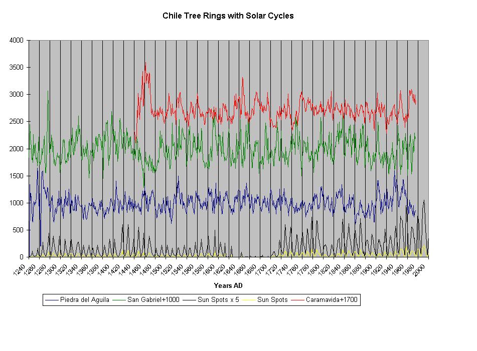
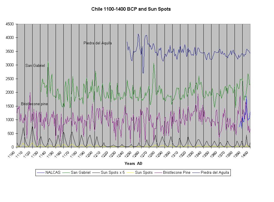
Dr. William Quinn of Oregon State University in the book  El Niño (1993) edited by Diaz and Markgraf made the connection between  El Niño events and the height of the Nile flood.  He used Nilometer data from 622 to 1900 AD (Arabic 0 AH) an showed that drought and low Nile readings happened because of low rain in Central Africa  with every recorded El Niño and that high floods happened with strong La Niña events. But Both El Niño and La Niña events also are recorded in tree ring data back to 7000 BC. Taking the tree ring data and the Palmero stone flood data, linking the times on the fragments based upon reconstruction of the whole monument,  we are able to synchronize these events and there is one and only one pattern that fits the whole “fingerprint” presented.  This happily matched the best estimates done by E. Edwards in Cambridge Ancient History very well,  with only about 4 to 10 years “slip” necessary between the patterns to make them match.  There also was one fingerprint which was unusual; and extra large high with three lows,  which is unique in the time span as well as other things which assure that we have a right match.

Thus we are able here to present absolute chronology for the first time with high confidence by use of tree rings,  ENSO events and known Nile river flood levels. As a side note the tree rings really are offset by one year since they include a zero years which does not mach, 1 BC is followed by 1 AD without zero, but that is inconvenient for people who work with dendrochronology so they offset to include a zero. Thus a one year correction must be made for that.  Also we can use all the other data such as known spans, etc. to fit the whole pattern from about 3300 to 2300 BC within a one year probable maximal deviation.

DENDROCHRONOLOGY

AS has been discussed above Dendrochronology (thee ring growth patterns) correlate well with El Niño and La Niña events, and  also with sun spot cycles which are believed to be the driving force for the set of events. This is reinforced by tree rings from Germany (Sepssart and Trier Forests) Java, Chile (not shown)  etc.. world wide; they all show synchronous patterns. This is shown below. Note that the data really needs to be expanded to see detail and that a rather massive file for Bristlecone pine which is continuous for 7000 unbroken years is a master file- It is some what tedious, and is broken into two files for minimization of problems, one file 5022 rows by 22 columns going back  to 3000 BC , and another that carries from about 3000BC back to 5000BC.

The solar cycles s and El Nino events also have been deduced for t he entire range, extending our map of solar cycle for MUCH longer than direct observation will allow.